Here’s a template which I created with the help of a few friends, a Senior Destinations Spreadsheet, which lets you and your group of friends share where you decide to go after high school. Of course, there are more applications of this than just that, but this is its intended use and audience.
Above is a preview of what this spreadsheet is capable of.
The Template Spreadsheet
https://docs.google.com/spreadsheets/d/1_8ANE6vwHf-0tyk1zu6KrvQLHPJXb_bswFbL0kd3dAE
To use it, all you have to do is go to File > Make a Copy. If that option is grayed out, that means you haven’t logged into your Google Account. Log into that, then click Make a Copy.
Instructions
To use this sheet, all you have to do is copy/paste in a list of names into column A, then type in each student’s respective college and the college’s city. Use the tabs located at the bottom of the webpage in order to navigate between the various pre-formatted sheets. That’s it.
Be sure to delete the example data beforehand, and also update the name of your spreadsheet by removing “(Template)” and adding your class number, such as “Class of 2023” or whatever name you want to name it.
Google Sheets formulas will automatically sort your data, so don’t modify those unless you know what you’re doing.
Locations:
If the location of the college is in the U.S., then input the location as “City, State”, but with the abbreviated state (such as WA or CA).
There is one exception to this rule, and that is when dealing with colleges located in Washington D.C., in that case, type in the state as “D.C.” (including the periods).
If the location of the college is not in the U.S., then input the location as “City, Country” without any abbreviations.
Note:
Inserting a new row for this spreadsheet requires a special process. If you want to insert a new row, follow these simple steps to ensure that the spreadsheet doesn’t break.
- Right-click on a row number on the left side, and select “Insert 1 Above” or “Insert 1 Below”
- Then, right-click on the row number on the left side of an already existing row, and copy it (Ctrl/Cmd + C)
- Then, right-click on the row number of your newly created row, and paste it (Ctrl/Cmd + V)
The reason we have to do this because this sheet relies on the right-most side’s columns (helper columns), from column Y through column AC.
If you want to delete a row, then all you have to do is right-click on any row number, and click “Delete Row”.
Troubleshooting:
- Double check your spelling. Spelling of locations are very important.
- When inserting new rows, make sure that the named ranges are still okay, and have not randomly skipped over a person. You can check this via Data > Named Ranges.
Features of this Spreadsheet
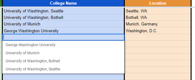
Dropdown Menus For College Name and Location
This feature creates a dropdown menu which takes a list of all the other entries in the row and updates it as new data is being inputted. This helps out when spellchecking, because you can just select an already-existing selection.
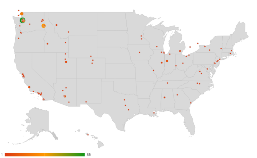
Automatic Map Plotting
Using the mapping feature of Google Sheets, we are able to place a dot based on where your college is. These maps rely heavily on correct spelling, so please make sure to spell your places correctly, and also to specify the location if necessary. For example, there are multiple campus locations for “University of Washington” so be sure to specify the correct campus, or else Google will automatically plot a default location.
Use the tabs at the bottom of the spreadsheet to navigate between the different maps. Google decides to repopulate the map each time it’s loaded, so use an external website such as https://www.easymapmaker.com/ in order to make a map which has almost no loading time.
Here’s what our map we ended up with looked like. The red dot at the very bottom of the U.S. map is “Universidad Anáhuac Mexico North Campus” which is why it’s plotted where Mexico should be, and a few red dots not on the U.S. because they are in Canada.

Here’s what our world map looked like:

Clearly, most of the 500ish people in my grade at my school stayed in the U.S., which was not really that surprising.
Data Sorting and Easy Exporting
Heading over to the #MapData tab, we can see that all of the inputted data is automatically sorted and easy to paste into other mapmaking tools.
Do not ever edit anything the #MapData tab, unless you know what you are doing. Everything on that page is formulas. Editing parts of this page may cause errors to occur.
The first three columns A-C alphabetically sorts the data based on the name of the college, and lists out the names of the students in a comma-seperated list, in order of increasing row number.
The next three columns E-G alphabetically sorts the data based on the location, and lists the names of the students in a comma-seperated list, in order of increasing row number.
Columns I-J count the number of students which are going to each state.
Columns L-M count the number of students which are going to each country.
All of this data can be easily copy/pasted to another program or website.
Accidental Edit Warnings
I set up the spreadsheet to warn you if you try to edit the contents of any tab other than the “College List” tab. This is to prevent any formulas from accidentally breaking. The “College List” sheet can still be broken if the formulas on the very right are edited, so be careful with those, because that is the only tab without protected ranges (lock icons in the tabs).
If you want to edit or remove those accidental edit warnings, or want to modify the permissions to only allow yourself to edit, then:
- Right click on the tab whose permissions you want to modify.
- Select “Protect sheet”.
- Select “Cancel”
Now you can see the current settings of the sheet. You can modify the permissions from there.
We clicked “Cancel” because the individual pages should already have permissions set up already, and we don’t want to double up on setting permissions.
Extra Trailing Space Checker
Using Google Sheets Data Validation, I set the spreadsheet up to mark any College Name or College Location with extra trailing spaces with a red tick mark in the corner.
This ensures that there are no duplicate entries in the #MapData sheet, because trailing spaces cause lots of problems.
In this example photo, I added a space after “George Washington University” and “Munich, Germany” in order to show off this feature.
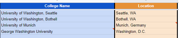
A cell with an empty space in it is also marked with a red marker.
Hope this template works well! Please contact me if you have any questions, notice any mistakes, or want to see a feature implemented.