Birthday Calendar Template (Google Sheets)

Hey everyone, I’d like to share with you this amazing birthday calendar I’ve created via Google Sheets!

Instructions

Also, here are some instructions on how to use it:

Make a copy (File → Make a Copy)
- Make sure you’re logged in using a Google Account or the button will be greyed out
Input the names and birthdays (years are not necessary), a red marker will indicate months spelled incorrectly and invalid dates.
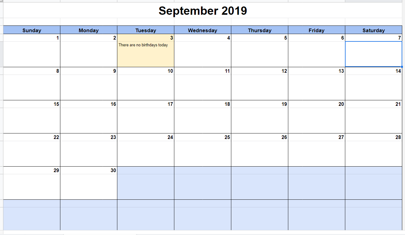
The #Birthday #Calendar should automatically update and change based on the current month.
The Now? column (D) will display a crown if their birthday is today.
You can adjust the settings of the calendar to fit your needs. They are there to help you if you want to print your calendar, and want certain features removed.
You can change the title of the calendar (A1 of the #Birthday #Calendar sheet, however, you’ll need to put your own formula in if you want it to update automatically depending on the month. I’ve put in a few preset ones, but you can change it if you’d like.
Names without a birthday will not be displayed.

How The Sheet Works

The Dynamic Calendar

The calendar I made by using BenAtShaw’s video, which I modified to fit these needs. It’s not exactly the same as his, but I used his to base this design off of. There are a lot of conditional formatting going on in this sheet.

Calendar Conditional Formatting (Coloring)

For the ranges A4:G4,A6:G6,A8:G8,A10:G10,A12:G12,A14:G14 I use the following custom formula: =ABS(A4)=0 to make those cells blue, which is what BenAtShaw did. To make those same cells yellow to highlight the day today, I use the custom formula: =AND(DAY(TODAY())-A4=0,$H$6=”Yes”). The $H$6=”Yes” part is the settings asking whether you want today to be highlighted. If it’s on “No”, then it won’t be highlighted.

Similarly, the ranges A5:G5,A7:G7,A9:G9,A11:G11,A13:G13,A15:G15 use the exact same formulas as above.

In case you’re curious, the colors I used were the yellow color preset “light yellow 3” and the blue I used was a custom shade of blue with RGB values of 217, 229, 252.

Filling the Calendar with Birthdays

Well, I wrote this very simple query formula to query the birthdays. This formula came from A5 of the #Birthday #Calendar sheet.

=IFERROR(IF(ABS(A4)=0,“”,JOIN(” “,QUERY(Database,“select Z where A is not null and Y = “&DATEVALUE(A4&” “&$H$7)))),IF(DAY(TODAYDATE)–A4=0,IF(Database!$H$7=“Yes”,“There are no birthdays today”,“”),“”))

Basically, what this does is it querys the Database, which is another named range which contains the entire Database sheet. The query basically displays column Z, which is the formatted display where the birthday is equivalent to that day. If it can’t find anything, it will output an error, which is why I put an IFERROR to catch it and display, according to the settings, either “There are no birthdays today”, or leave the cell blank.

Calculating Ages

To calculate the ages of the people to be displayed, I came up with the following formula (from Z2 of the Database sheet):

=IFERROR(IF($H$5=“Yes”,IF(AND(NOT(ABS(B2)=0),ABS(C2)=0),IF($H$12=“(??)”,A2&” (??)”,A2),A2&” (“&DATEDIF(CONCATENATE(TEXT($B2,“mm/dd”), “/”, $C2), TODAYDATE+31, “Y”)&“)”),A2),“”)

Yeah, it’s kind of long, but basically what it does is it takes the difference between the two dates and formats it accordingly to your setting choice. If there’s no year, it will either display the name of the person with a “(??)” instead of an age, or it will display just their name, depending on the setting you chose. TODAYDATE is a named range which contains the formula =TODAY() for optimization purposes. I use the date difference (DATEDIF) between their birthday and today + 31 days so that it can calculate the age of the people at the end of the month correctly when it’s still the beginning of the month.

The Now? Column

The Now? Column basically displays a crown whenever today is their birthday. It uses a very simple formula that I came up with (from D2 of the Database sheet):

=IFERROR(IF(DATEVALUE(B2)=DATEVALUE(TEXT(TODAYDATE,“mm/dd”)),“♛”,“”),“”)

Basically, it checks if the Month+Day column (B) has the same date as today. If it does, then it will display a crown. If not, then it won’t.

Settings

With the settings, creating the dropdown menus were pretty simple. If you don’t know how to do so, right click on the cell you want dropdown menus for, and select Data Validation. 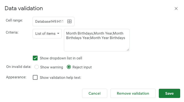That is how I created the dropdown menus by checkmarking the box that says Show dropdown list in cell and putting a list of items down. How to make the settings actually do something is by using a bunch of IF statements to see which of the options were chosen. For example, this is the formula I used to display the title of the birthday calendar (from A1 of the #Birthday #Calendar sheet):

=IF(Database!H9=“Month Year Birthdays”,TEXT(TODAYDATE,“MMMM YYYY Birt\h\da\y\s”),IF(Database!H9=“Month Birthdays”,TEXT(TODAYDATE,“MMMM Birt\h\da\y\s”),IF(Database!H9=“Month Year”,TEXT(TODAYDATE,“MMMM YYYY”),TEXT(TODAYDATE,“MMMM Birt\h\da\y\s YYYY”))))

It’s really simple, but looks complicated because there were 4 different options to choose from. Hope this gives you some insight into how I created this amazing Birthday Calendar spreadsheet!