In this article, I will list many of the date functions you’ll need to do basic things.
There are a few things you need to know as dates.
Date Values
Each date, for example, October 24, 2018, has an assigned Date Value, which in this case, is 43397. The Date Value’s “0” value is on December 30th, 1899. The Date Value increments by 1 per day, and it can go into the negatives. For example, January 1st, 1800 is -36522. These Date Values will be handy in the future.
However, let’s begin by discussing the format of dates.
Date Formats
If you type in =TODAY() into any cell, you’ll end up getting the day’s date you type in with the format of “mm/dd/yyyy” and the output “10/24/2018”, assuming you live in the US. If you want to change the formatting of the cell, just head over to the “Format” tab and you have a bunch of options to choose from.
 But let’s say you’re lazy and don’t want to bother with the formatting tab, or you don’t like any of the preset formats. Well, you can create your own formats using the TEXT() function.
Type in the Date Value into the number slot and type in your format in quotes in the format section. Remember that TODAY() counts as a Date Value.

Here are a few examples of formats. The letter “m” is used for months.
| Cell Input | Output | Description |
| =TEXT(TODAY(),“m”) | 9 | The month number in a year (1 = January, 2 = February), with numbers 0 to 9 being one character long |
| =TEXT(TODAY(),“mm”) | 09 | The month number in a year, always has length 2 |
| =TEXT(TODAY(),“mmm”) | Sep | The month name shortened to 3 letters |
| =TEXT(TODAY(),“mmmm”) | September | The full month name |
| =TEXT(TODAY(),“mmmmm”) | S | The first letter of the month |
| =TEXT(TODAY(),“mmmmmm”) | September | Any more m’s just output the full month name. |
Likewise, you can do the same thing with years and days. The letter “y” is used for years, “d” for days. For example, “dd” would output 12 and “ddd” would be Fri for Friday.
“m” for minutes, “s” for seconds, and “h” for hours.
Escape Sequences
| Cell Input | Output |
| =TEXT(TODAY(),“mm/dd/yy”) | 09/12/18 |
| =TEXT(TODAY(),”dd/yyyy/mmm”) | 12/2018/Sep |
| =TEXT(TODAY(),”Today is: dddd”) | To12a18 i0: Wednesday |
| =TEXT(TODAY(),”To\da\y i\s dddd” | Today is Wednesday |
If the format contains any of the characters m, d, y, s, or h, it will take it as a thing to replace. However, if you for some reason want to include those characters in the format, you have to type in a “\” before the character, as shown in the fourth example above. This backslash is known as an escape sequence. If you wanted to include the backslash in your format, then you would need to type in “\\” to output a “\” (similar to coding in Java).
Date Differences
If you wanted to calculate the difference between certain dates, you’d use the function =DATEDIF().
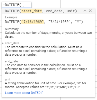 The start_date and end_date are pretty self-explanatory, just type them in using quotes. You can also type in, for example, TODAY() as your start date. The unit‘s are the only tricky spot in this situation.
Units
- “D” counts the number of days between the start and end. If your starting date is 10/24/2018 and your end date was 10/25/2018, the output would be 1. If your starting date is 10/24/2018 and your end date is also 10/24/2018, then the output would be 0. Make sure that the start date is before the end date otherwise you’ll get an error.
- “M” counts the whole number of months between the start and end, rounded down. Months are calculated by the day number in each month (so months with 28 days, 30 days, and 31 days affect the calculation). If the first date is 9/12/2018 and the end date is 10/12/2018, then that would count as 1 month. Same goes for 2/28/2018 and 3/28/2018. Even though there are 28 days in between them, instead of 30, it still counts as 1. If the start is 2/28/2018 and the end is 3/27/2018, it would output 0, since less than a whole month has passed.
- “Y” counts the whole number of years between the start and end.
DateDif Examples:
An example of using DATEDIF is: =DATEDIF(“2018-2-28”,“2018-3-28”,“D”) and the output will be 28, as 28 whole days are in between those two dates.
For example, given the birthday of someone, we can calculate their age.
If C69 contains “January 1” and D69 contains “1995”, then we can calculate how old they are (as of November 7, 2018): 23 Years, 10 Months, 6 Days old.
=IF(AND(NOT(ISBLANK(C69)),NOT(ISBLANK(D69))),(DATEDIF(CONCATENATE(TEXT($C69,“mm/dd”), “/”, $D69), TODAY(), “Y”) & ” Years, “ & DATEDIF(CONCATENATE(TEXT($C69,“mm/dd”), “/”, $D69), TODAY(), “YM”) & IF(DATEDIF(CONCATENATE(TEXT($C69,“mm/dd”), “/”, $D69), TODAY(), “YM”) = 1, ” Month, “, ” Months, “) & DATEDIF(CONCATENATE(TEXT($C69,“mm/dd”), “/”, $D69), TODAY(), “MD”) & IF(DATEDIF(CONCATENATE(TEXT($C69,“mm/dd”), “/”, $D69), TODAY(), “MD”) = 1, ” Day”, ” Days”)),“”)